Conditional Formatting#
Cell style can change based on conditional rules. Conditional rules are written as formulas. Conditional formatting can apply to an entire row or cells in a column.
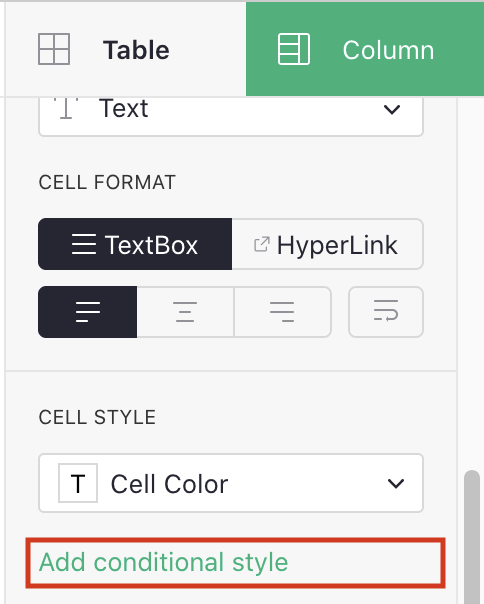
To add conditional formatting to a particular column, select the column, go to the CELL STYLE section of the creator panel under the Column tab, and click on Add conditional style.
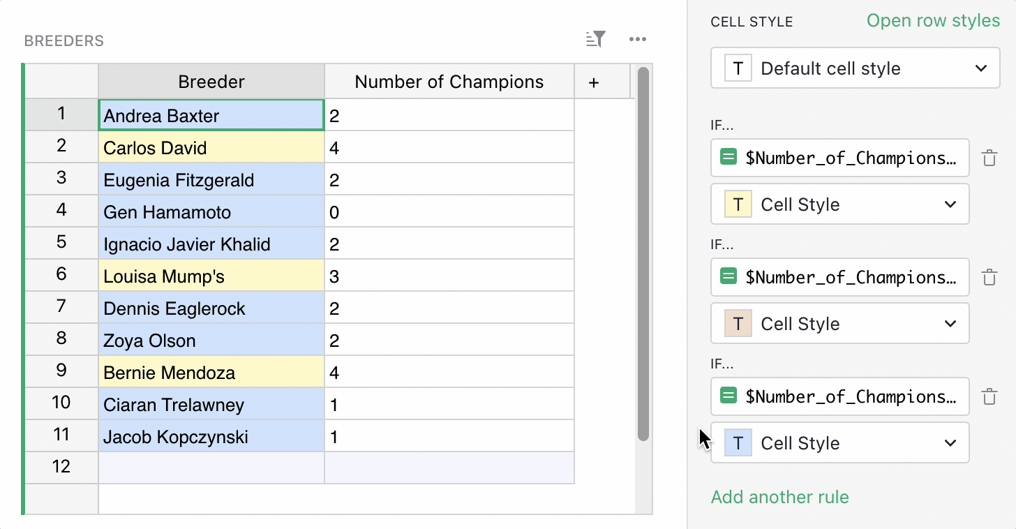
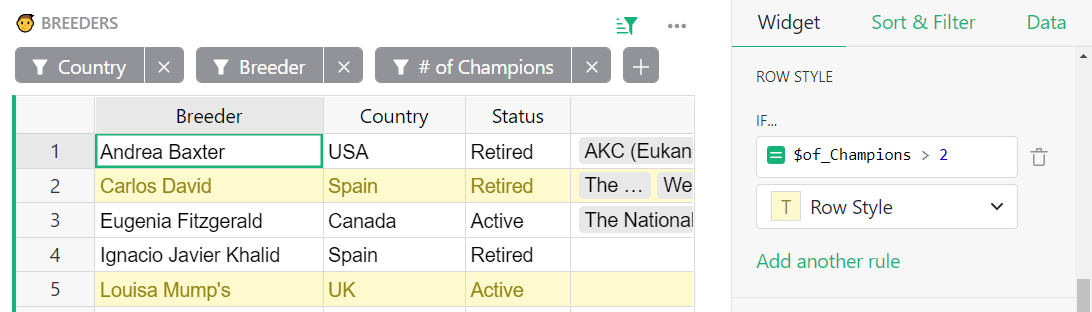
In this example, we have a list of dog breeders who have raised champion thoroughbreds. Let’s apply conditional formatting to the Breeder column based on the number of champion dogs. We would like to highlight in gold any breeders with more than 2 champions.
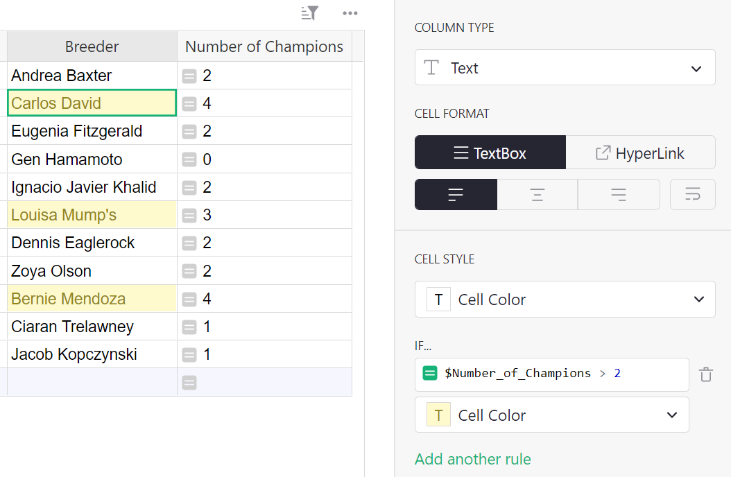
Here the conditional formula is $Number_of_Champions > 2.
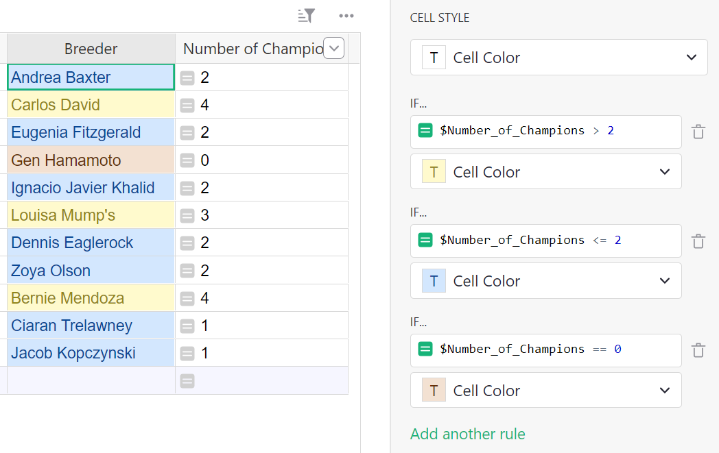
We would also like to highlight breeders with 1 or 2 champion dogs in blue, and 0 champion dogs in brown. Click Add another rule to add more conditional styles.
To add conditional formatting to rows, go to the ROW STYLE section of the creator panel under the Table > Widget tab, and click on Add conditional style.
Order of Rules#
Note that Grist applies the rules in order from top to bottom. Styles applied by rules that appear later in the list will override those applied by rules earlier in the list. To change the order of the rules, hover over a rule to reveal a drag handle, then click and drag the handle to move the rule to its new position.
What would happen if we swapped the last two rules in the example above?
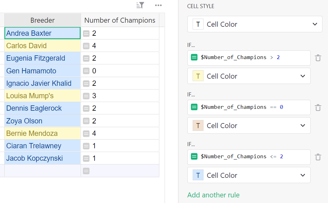
Notice that Gen Hamamoto, who has 0 champion dogs, is not highlighted in brown. This is because after applying the second conditional style, $Number_of_Champions == 0, Grist applied the third, $Number_of_Champions <= 2, which applies to Gen Hamamoto as well and shades him blue. When we change the order of the rules so that the second and third conditional styles switch positions, Gen Hamamoto will be highlighted in brown.